Quasi Cauchy Optimizer

This article contains some notes about the quasi Cauchy optimizer implementation. The discussed method is a member of the quasi Newton family. It minimizes a function \(f(x)\) which maps an n-vector \(x\) to a scalar, where \(f(x)\) could be a loss function used in machine learning algorithms. The Hessian is approximated by a diagonal matrix satisfying the weak secant equation. Because a diagonal matrix has the same memory footprint as a vector, the method is well suited for high-dimensional problems (e.g. neural networks).

Weak Secant Equation

The weak secant equation is \(s^{T} \cdot y= s^{T} \cdot B_{+} \cdot s\) with the update step \(s=x_{+}-x\), the gradient difference \(y=\nabla f(x_{+})-\nabla f(x)\) and \(s^{T} \cdot y \gt 0\). The \(n \times n\) matrix \(B_{+}\) is an approximation of the Hessian of \(f(x)\) which satisfies the weak secant equation. Like in Newton's method, the update step is \(s=-B^{-1} \cdot \nabla f(x)\) where the steepest-descent direction \(-\nabla f(x)\) is scaled and rotated by \(B^{-1}\). For more details see the paper of Zhu et al.

Scaled Identity Update

We can use a scaled identity matrix \(D=d \cdot I\) for the Hessian approximation \(B_{+}\). Inserting into the weak secant equation, this gives \(s^{T} \cdot y= s^{T} \cdot d \cdot I \cdot s\). Solving for the scalar \(d\) we get \(d=\frac{s^{T} \cdot y}{s^{T} \cdot s}\). This Hessian approximation uniformly scales all steepest-descent dimensions by \(\frac{1}{d}\) in the update step.

Diagonal Update

Instead of the scaled identity matrix, we can also use a diagonal matrix \(D\) for the Hessian approximation. There is not a unique solution for a diagonal matrix, so we narrow down the solution \(D_{+}\) to be the one most similar to the previous matrix \(D\). The similarity is measured as: \[\| D_{+}-D \| = \| U \| = \sqrt{\sum_{i}{u_{ii}^2}} \] By taking the smallest possible update \(U\), this keeps as much information as possible from previous iterations. This gives the optimization problem \(min \| U \| \) with the weak secant equation \(s^T \cdot (D+U) \cdot s = s^T \cdot y\) as constraint. The Lagrange function is: \[L(U, \lambda) = \frac{1}{2} \cdot \| U \|^2 + \lambda \cdot (s^T \cdot (D+U) \cdot s - s^T \cdot y) \] Computing the partial derivatives with respect to the diagonal elements \(u_{ii}\) and \(\lambda\) and setting them to zero gives the update: \[u_{ii} = \frac{s^T \cdot y - s^T \cdot D \cdot s}{\sum_{j}{s_j^4}} \cdot s_i^2\] This Hessian approximation scales each steepest-descent dimension individually by \(\frac{1}{u_{ii}}\) in the update step.

Experiments

The results can be reproduced with the quasi Cauchy optimizer implementation. The implementation uses line-search. Further, it clips the Hessian approximation to positive values as a crude way to ensure moving along a descent direction. Here only a small subset of the results is shown. Comparing the diagonal update and the scaled identity update on multiple test-functions shows the following:

• The typical test-functions (Beale, Rosenbrock, ...) have a low number of dimensions, and for these functions the scaled identity update performs better (see Fig. 1 and Table 1)
• For high-dimensional functions with scale varying across dimensions, the diagonal update performs better (see Table 2)

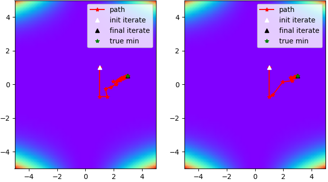Fig. 1: Path towards the minimum of the Beale test-function. Left: diagonal update. Right: scaled identity update.

Update	Error	Iteration Count
Diagonal	0.000	172
Scaled Identity	0.000	33

Table 1: Beale test function.

Update	Error	Iteration Count
Diagonal	0.383	185
Scaled Identity	0.649	501 (max. reached)

Table 2: 50-dimensional polynomial.

Conclusion

The diagonal update derived from the weak secant equation scales each steepest descent dimension separately. This update performs better for high-dimensional functions with scale varying across dimensions. Otherwise, uniform scaling performs better.

Harald Scheidl, 2020